Data Science for Agentic AI
MSA 8700 — Module 11
Business Analogy:
Clickstream / Customer Journey Analytics
Discussion Prompt: “What does a ‘bounce’ look like in an agent system? Is it always bad? When might a single-step completion be desirable, and when does it signal a problem?”
Business Analogy:
KPI Trend Monitoring / Demand Forecasting / SLA Tracking
Quality Metrics Over Time
Track these as time series:
- Answer correctness (human-rated or LLM-judged on a sample)
- Task success rate (binary: did the agent complete the task?)
- Latency (end-to-end and per-step)
- Token consumption (cost proxy)
- User satisfaction (if feedback is collected)
Time-Series Analysis
Apply standard decomposition: trend (is quality declining?), seasonality (do certain times of day or week show different performance — e.g., batch jobs competing for GPU resources?), residual (noise vs. signal). Rolling averages (7-day, 28-day) smooth noise and reveal trend.
Statistical Process Control (SPC)
Control charts — X-bar, R-charts, CUSUM — are used identically in manufacturing QA, service level monitoring, and agent performance tracking. The logic:
- Establish a baseline period of stable performance.
- Compute control limits (typically ±3σ).
- Plot ongoing metrics against these limits.
- Flag violations: single point outside limits, runs of 7+ above/below center, trending sequences.
CUSUM (Cumulative Sum) charts are particularly valuable for detecting small, sustained shifts — the kind of slow degradation that agents exhibit when upstream data changes or model weights drift subtly.
Change-Point Detection
Algorithms like PELT (Pruned Exact Linear Time) or Bayesian Online Change-Point Detection identify the moment a distribution shifts. In manufacturing, this detects when a machine tool begins producing slightly out-of-spec parts. In agent systems, it detects when answer quality shifts — perhaps because the retrieval index was updated, a model version changed, or the distribution of user queries evolved.
Concept Drift
Concept drift in business forecasting occurs when the relationship between features and target changes — a demand model trained in 2024 underperforms in 2025 because consumer behavior shifted. In agent systems, the equivalent is task distribution drift: the queries users ask evolve, the documents in the knowledge base age, or the external APIs the agent calls change their response format. The agent’s behavior degrades not because the agent changed, but because the world did.
Key Insight: “How do you know your agent got worse before your users tell you?” The answer is the same as in any business: instrument the process, track the metrics, set control limits, and automate anomaly detection. SPC is not a manufacturing technique — it is a process monitoring technique that applies to any repeated operation.
Business Analogy:
Customer Complaint Classification / Fraud Detection / Ticket Routing
Taxonomy of Agent Failures
Agent outputs fail in categorizable ways. A working taxonomy:
| Failure Category | Description | Business Analogy |
|---|---|---|
| Hallucination | Agent generates factually incorrect content with high confidence | Fraudulent transaction — looks legitimate, isn’t |
| Tool failure | External tool returns an error or unexpected result | Supply chain disruption — upstream dependency fails |
| Misrouting | Agent selects the wrong tool or wrong sub-agent for the task | Ticket misrouted to the wrong department |
| Context loss | Agent loses track of conversation history or task state | Customer has to repeat their problem to a new rep |
| Prompt injection | Adversarial input causes the agent to deviate from instructions | Social engineering attack on a call center agent |
| Infinite loop | Agent enters a cycle of repeated actions without progress | Escalation loop — ticket bounces between departments |
| Partial completion | Agent completes part of the task but misses key requirements | Order shipped incomplete |
Multi-Label Classification
A single agent output can exhibit multiple failure modes simultaneously — a hallucinated answer that also lost context and was produced after a silent tool failure. This is a multi-label classification problem, not multi-class. The distinction matters for metric selection (use Hamming loss, subset accuracy, or per-label F1 rather than simple accuracy).
Cost-Sensitive Classification
The cost asymmetry is severe and asymmetric — exactly as in fraud detection:
- False negative (missed hallucination): User acts on incorrect information. Reputational damage, safety risk, liability. High cost.
- False positive (flagged a correct answer as hallucination): Answer gets reviewed unnecessarily. Human effort wasted. Low cost.
This asymmetry demands threshold tuning, class weighting, or cost-sensitive loss functions — the same toolkit used in fraud detection, medical screening, and safety-critical classification.
The Label Definition Problem
Key Insight: Deciding what counts as “failure” is a domain problem, not a modeling problem. This is identical to the challenge of defining “churn” in a CRM system (inactive for 30 days? 60 days? Reduced usage? Canceled subscription?) or defining “fraud” in a payments system (rule-based threshold? Statistical anomaly? Confirmed investigation?). The taxonomy above is a starting point — every deployment will require domain-specific refinement based on the use case, the user population, and the consequences of each failure type.
Active Learning for Efficient Labeling
Agent failure labels are expensive to obtain — they require expert review of each output. Active learning addresses this by prioritizing the most informative examples for labeling:
- Uncertainty sampling: Label the examples where the current classifier is least confident — exactly the strategy used to efficiently label rare fraud cases or ambiguous medical images.
- Query-by-committee: Multiple models vote; label the examples where they disagree most.
The result: a usable classifier with far fewer labeled examples than random sampling would require.
Confusion Matrix Walkthrough
Consider a binary “hallucination detector” evaluated on 500 agent outputs:
| Predicted: Hallucination | Predicted: Correct | |
|---|---|---|
| Actual: Hallucination | 38 (TP) | 12 (FN) |
| Actual: Correct | 25 (FP) | 425 (TN) |
- Precision: 38/63 = 60% — many flagged outputs are actually fine.
- Recall: 38/50 = 76% — 24% of hallucinations slip through.
- For this use case, recall matters more. A missed hallucination is costlier than a false flag. Tune the threshold to push recall toward 90%+ even at the expense of precision — same reasoning as in fraud detection.
Discussion Prompt: “In your own agent system, what failure categories would you define? How would you decide the boundary between ‘partially correct’ and ‘failure’?”
Business Analogy:
Search Relevance / Recommendation Systems / Catalog Coverage
The Metrics
RAG system retrieval quality is evaluated with the same metrics used in e-commerce search and recommendation engine evaluation:
- Precision@k — Of the top-k retrieved documents, how many are relevant? (Same as: of the top-k search results on an e-commerce site, how many match the shopper’s intent?)
- Recall@k — Of all relevant documents in the corpus, how many appear in the top-k? (Same as: does the search engine surface all relevant products, or miss some?)
- NDCG (Normalized Discounted Cumulative Gain) — Are the most relevant documents ranked highest? (Same as: are the best products at the top of the search results page?)
Retrieval Scores as Predictive Features
A natural analytical question: does retrieval similarity score predict answer quality? This is a regression / correlation analysis problem. Extract features from retrieval:
- Top-1 similarity score
- Mean and variance of top-k scores
- Gap between top-1 and top-2 scores (confidence margin)
- Chunk length of retrieved documents
- Query-document lexical overlap
Fit a regression model predicting answer quality (human-rated or LLM-judged) from these features. The feature importance ranking tells you which aspects of retrieval matter most for downstream quality — actionable intelligence for tuning the retrieval pipeline.
Coverage Analysis
Which query clusters have poor retrieval performance? Embed user queries, cluster them (K-means or HDBSCAN), and compute per-cluster retrieval metrics. This reveals underserved segments — query types where the knowledge base has gaps or the embedding model performs poorly.
This is identical to identifying underserved customer segments in retail analytics: which customer cohorts have low conversion rates? What products are they searching for that the catalog doesn’t carry?
Key Insight: RAG quality is a regression problem. Predict answer quality from retrieval features, identify the weak spots, and invest in the clusters where retrieval fails. The analytical framework is identical to diagnosing why certain customer segments have poor conversion on an e-commerce site.
Business Analogy:
Call Center Workforce Management / Supply Chain Optimization / Hospital Patient Flow
Agent Pipelines as Queuing Systems
A multi-agent system is a queuing network. Queries arrive, wait for an available agent instance, get processed through a sequence of steps (sub-agents, tools, LLM calls), and exit. This is structurally identical to:
- A call center: calls arrive, wait in queue, get handled by agents, transfer between departments.
- A hospital emergency department: patients arrive, triage, wait, get treated by specialists, discharge.
- A supply chain: orders arrive, get processed through manufacturing stages, ship.
Little’s Law
L = λW
- L = average number of tasks in the system (in-progress)
- λ = average arrival rate (queries per second)
- W = average time a task spends in the system (end-to-end latency)
This holds for any stable queuing system. If your agent handles λ = 5 queries/minute and each takes W = 30 seconds on average, you’ll have L = 2.5 tasks in-flight on average. If W increases to 60 seconds, L doubles — and if you only have 3 agent instances, the queue begins to grow.
Little’s Law is taught in every operations management course. It applies to agent systems without modification.
Bottleneck Identification
Theory of Constraints (TOC): The throughput of the entire system is limited by its slowest component. In a multi-agent pipeline:
- Measure utilization of each sub-agent and tool: utilization = (busy time) / (total time).
- The component with the highest utilization is the bottleneck.
- Improving any non-bottleneck component has zero impact on system throughput.
This is the same analysis used to identify the bottleneck station in a manufacturing line or the overloaded department in a call center.
Service Time Distributions
Tool call durations and sub-agent processing times are rarely normally distributed. They typically follow Log-Normal or Gamma distributions — a long right tail with occasional slow calls. Fitting the correct distribution matters for:
- Capacity planning (how many instances do you need to meet SLA at the 95th percentile?)
- Anomaly detection (is a 45-second tool call genuinely unusual, or just the tail of the distribution?)
This is the same distributional modeling used for service times in retail checkout, hospital procedure durations, and warehouse pick times.
Visualization
Gantt-style charts of parallel agent execution reveal the critical path — the longest sequential chain of dependencies that determines end-to-end latency.
This is identical to critical path analysis in project management.
- Shorten the critical path → shorten total latency
- Shorten a non-critical parallel branch → changes nothing
Discussion Prompt: “In your own agent system, which component do you suspect is the bottleneck? How would you measure it? What would you do if you confirmed it?”
Business Analogy:
A/B Testing / Marketing Campaign Experiments / Clinical Trials
Controlled Experiments for Agents
To compare agent configurations (different models, prompts, tool sets, retrieval strategies), run a controlled experiment:
- Hold the task set constant — use a fixed evaluation benchmark of representative queries.
- Vary one configuration dimension at a time (or use factorial design for interactions).
- Randomize the assignment of queries to configurations to avoid selection bias.
This is standard A/B testing methodology, applied to agent configurations rather than website layouts or ad copy.
Statistical Significance Testing
Compare quality scores between configurations:
- t-test (or Welch’s t-test) when quality scores are approximately normal.
- Mann-Whitney U test when distributions are skewed or ordinal — common with Likert-scale ratings or LLM-judged scores.
- Paired tests when you can run both configurations on the same queries (within-subjects design) — more statistical power.
' stroke='%23e74c3c' stroke-width='1.5'/%3E%3Cpath d='M70,60 C85,60 100,58 115,52 C130,42 140,28 155,22 C170,28 180,42 195,52 C210,58 230,60 250,60' fill='rgba(46,204,113,0.3)' stroke='%232ecc71' stroke-width='1.5'/%3E%3Cline x1='105' y1='14' x2='105' y2='60' stroke='%23e74c3c' stroke-dasharray='3,3'/%3E%3Cline x1='155' y1='18' x2='155' y2='60' stroke='%232ecc71' stroke-dasharray='3,3'/%3E%3Ctext x='105' y='68' fill='%23e74c3c' font-size='7' font-family='sans-serif' text-anchor='middle'%3Eμ_A%3C/text%3E%3Ctext x='155' y='68' fill='%232ecc71' font-size='7' font-family='sans-serif' text-anchor='middle'%3Eμ_B%3C/text%3E%3Cline x1='110' y1='38' x2='148' y2='38' stroke='white' stroke-width='1'/%3E%3Cpolygon points='148,36 154,38 148,40' fill='white'/%3E%3Ctext x='130' y='35' fill='%23ccc' font-size='7' font-family='sans-serif' text-anchor='middle'%3EΔ%3C/text%3E%3Ctext x='130' y='82' fill='%23ddd' font-size='10' font-family='sans-serif' font-weight='bold' text-anchor='middle'%3EMann-Whitney U — ranked scores%3C/text%3E%3Cline x1='15' y1='138' x2='250' y2='138' stroke='%23888'/%3E%3Cline x1='15' y1='88' x2='15' y2='138' stroke='%23888'/%3E%3Crect x='20' y='125' width='14' height='13' fill='rgba(231,76,60,0.5)' stroke='%23e74c3c'/%3E%3Crect x='38' y='118' width='14' height='20' fill='rgba(231,76,60,0.5)' stroke='%23e74c3c'/%3E%3Crect x='56' y='122' width='14' height='16' fill='rgba(231,76,60,0.5)' stroke='%23e74c3c'/%3E%3Crect x='74' y='114' width='14' height='24' fill='rgba(231,76,60,0.5)' stroke='%23e74c3c'/%3E%3Crect x='92' y='119' width='14' height='19' fill='rgba(231,76,60,0.5)' stroke='%23e74c3c'/%3E%3Crect x='120' y='110' width='14' height='28' fill='rgba(46,204,113,0.5)' stroke='%232ecc71'/%3E%3Crect x='138' y='104' width='14' height='34' fill='rgba(46,204,113,0.5)' stroke='%232ecc71'/%3E%3Crect x='156' y='96' width='14' height='42' fill='rgba(46,204,113,0.5)' stroke='%232ecc71'/%3E%3Crect x='174' y='102' width='14' height='36' fill='rgba(46,204,113,0.5)' stroke='%232ecc71'/%3E%3Crect x='192' y='92' width='14' height='46' fill='rgba(46,204,113,0.5)' stroke='%232ecc71'/%3E%3Ctext x='60' y='148' fill='%23e74c3c' font-size='7' font-family='sans-serif' text-anchor='middle'%3EConfig A%3C/text%3E%3Ctext x='163' y='148' fill='%232ecc71' font-size='7' font-family='sans-serif' text-anchor='middle'%3EConfig B%3C/text%3E%3Ctext x='130' y='160' fill='%23ddd' font-size='10' font-family='sans-serif' font-weight='bold' text-anchor='middle'%3EPaired test — same queries, two configs%3C/text%3E%3Cline x1='40' y1='166' x2='40' y2='200' stroke='%23888'/%3E%3Cline x1='220' y1='166' x2='220' y2='200' stroke='%23888'/%3E%3Ctext x='40' y='209' fill='%23e74c3c' font-size='7' font-family='sans-serif' text-anchor='middle'%3EConfig A%3C/text%3E%3Ctext x='220' y='209' fill='%232ecc71' font-size='7' font-family='sans-serif' text-anchor='middle'%3EConfig B%3C/text%3E%3Ccircle cx='40' cy='193' r='3' fill='%23e74c3c'/%3E%3Ccircle cx='220' cy='185' r='3' fill='%232ecc71'/%3E%3Cline x1='43' y1='193' x2='217' y2='185' stroke='%23666' stroke-width='0.8'/%3E%3Ccircle cx='40' cy='182' r='3' fill='%23e74c3c'/%3E%3Ccircle cx='220' cy='175' r='3' fill='%232ecc71'/%3E%3Cline x1='43' y1='182' x2='217' y2='175' stroke='%23666' stroke-width='0.8'/%3E%3Ccircle cx='40' cy='189' r='3' fill='%23e74c3c'/%3E%3Ccircle cx='220' cy='172' r='3' fill='%232ecc71'/%3E%3Cline x1='43' y1='189' x2='217' y2='172' stroke='%23666' stroke-width='0.8'/%3E%3Ccircle cx='40' cy='198' r='3' fill='%23e74c3c'/%3E%3Ccircle cx='220' cy='190' r='3' fill='%232ecc71'/%3E%3Cline x1='43' y1='198' x2='217' y2='190' stroke='%23666' stroke-width='0.8'/%3E%3Ccircle cx='40' cy='176' r='3' fill='%23e74c3c'/%3E%3Ccircle cx='220' cy='178' r='3' fill='%232ecc71'/%3E%3Cline x1='43' y1='176' x2='217' y2='178' stroke='%23666' stroke-width='0.8'/%3E%3C/svg%3E)
Effect Size
Key Insight: Statistical significance ≠ practical significance. A new retrieval strategy might produce a statistically significant 0.3-point improvement on a 100-point quality scale with p < 0.01 — and be completely irrelevant in practice. Always report effect size (Cohen’s d, or raw difference in meaningful units) alongside the p-value. This is the same lesson taught in every marketing experimentation course: a statistically significant 0.1% lift in click-through rate is real but may not justify the engineering effort.
Multi-Armed Bandit for Online Evaluation
When you cannot afford to commit 50% of traffic to a possibly inferior configuration for weeks, use multi-armed bandit algorithms (Thompson Sampling, UCB) to adaptively allocate traffic. Configurations that perform well get more traffic; poor performers get less. This is the same approach used in dynamic ad serving and personalized recommendation — exploit the best-known option while continuing to explore.
LLM-as-Judge: Measurement Instrument Validation
When using an LLM to judge agent output quality, treat the LLM-judge as a measurement instrument subject to the same validation requirements as a survey instrument in social science:
- Systematic bias: Does the judge favor longer answers? More formal tone? Answers that agree with its own knowledge?
- Calibration: Does a judge score of “4/5” mean the same thing across different query types?
- Inter-rater agreement: If you run the same judgment twice (or with two different judge models), how consistent are the scores? Compute Cohen’s kappa or Krippendorff’s alpha — the same metrics used to validate human annotation schemes.
Discussion Prompt: “If you were to run an A/B test on your own agent system, what is the single most important metric you would track, and how many queries would you need to detect a meaningful difference?”
Business Analogy:
Customer Segmentation / Market Basket Analysis / Behavioral Cohort Analysis
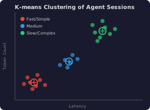
Clustering Agent Sessions
Represent each agent session as a behavioral feature vector: tool usage profile (which tools, how often), task length, latency, token count, outcome (success/failure), number of retries. Apply K-means, HDBSCAN, or Gaussian Mixture Models to discover natural groupings.
These clusters are agent behavioral segments — the equivalent of customer segments in CRM analytics.
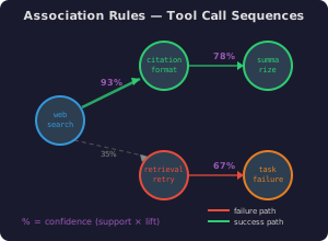
Association Rule Mining
Apply Apriori or FP-Growth to tool call sequences to discover frequent patterns: “When the agent calls web_search, it almost always calls citation_formatter next” or “Retrieval followed by a second retrieval attempt is associated with task failure.”
This is market basket analysis applied to agent behavior rather than shopping carts.
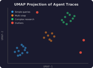
Dimensionality Reduction for Visualization
Embed agent traces (using their behavioral feature vectors or by embedding the full trace text) and project to 2D with UMAP or t-SNE. The resulting scatter plot reveals clusters, outliers, and structural patterns in agent behavior — a behavioral landscape map.
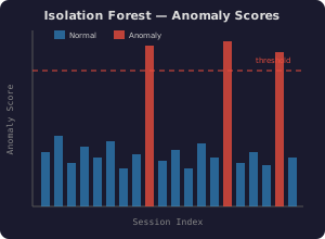
Outlier Detection
Isolation Forest, Local Outlier Factor (LOF), or DBSCAN’s noise points flag unusual agent sessions — sessions that don’t fit any normal behavioral cluster.
This is the same anomaly detection pipeline used in fraud analytics, network intrusion detection, and rare event identification in CRM.
Key Insight: Unsupervised methods are discovery tools. They answer the question you didn’t know to ask: “What behavioral patterns exist in my agent system that I haven’t designed for?”
Mapping Table
| Classic Analytics Problem | Agentic AI Equivalent | Key Technique |
|---|---|---|
| Conversion funnel analysis | Task completion path analysis | Sankey diagrams, sequence analysis |
| Concept drift in forecasting | Agent performance degradation | Change-point detection, SPC control charts |
| Customer complaint classification | Agent failure taxonomy | Multi-label classification, cost-sensitive learning |
| Search relevance optimization | Retrieval quality in RAG pipelines | NDCG, Precision@k, Recall@k |
| Call center queueing / workforce mgmt | Multi-agent coordination & load balancing | Little’s Law, utilization analysis, bottleneck ID |
| A/B testing marketing campaigns | Agent configuration experiments | t-test, Mann-Whitney U, effect size estimation |
| Customer segmentation | Agent behavioral clustering | K-means, HDBSCAN, UMAP |
| Fraud / anomaly detection | Unusual agent behavior detection | Isolation Forest, LOF, DBSCAN |
| Survey instrument validation | LLM-as-judge calibration | Cohen’s kappa, inter-rater reliability |
| Demand forecasting | Query volume & resource planning | Time-series decomposition, capacity models |
CASE STUDY:
The Struggling Research Assistant
The Struggling Research Assistant
System Description
A large research university has deployed an agentic AI research assistant to support graduate students across all departments. The system architecture:
- Retrieval pipeline: Semantic search (dense embeddings) over a corpus of 50,000 indexed academic papers
- Tools: Web search API, citation formatting tool, abstract summarization module
- LLM backbone: GPT-4-class model via API
- Deployment: 8 parallel agent instances behind a load balancer
- Volume: ~500 queries per day
The system has been running for 10 weeks. It was well-received at launch.
The Problem — Six Weeks Post-Launch
The following issues have been reported or observed:
- User satisfaction has dropped from 4.2/5 to 3.4/5 over six weeks (collected via post-interaction survey).
- Users report answers that “sound right but cite wrong papers” — the answers are fluent and plausible, but the cited sources do not support the claims made.
- Average response time has increased from 8 seconds to 22 seconds.
- Load imbalance: One of the 8 agent instances is handling approximately 60% of all queries. The other 7 share the remaining 40%.
- Silent retrieval failures: The retrieval tool is returning empty results (no documents found) for 12% of queries — but it does so without raising an error. The agent proceeds to answer without retrieved context.
Class Activity ACT11
Question 1 — Diagnose the Performance Drop
The satisfaction score declined from 4.2 to 3.4 over six weeks.
- What data would you collect to identify the root cause? Be specific about data sources (logs, metrics, traces, user feedback).
- What visualizations would you build to reveal the problem? Name the chart type and what it would show.
- Which of the five reported issues do you think is the primary driver of the satisfaction decline? Why?
- Map each reported issue to a specific data science technique covered in today’s session.
Question 2 — Design a Failure Classifier
Users report answers that “sound right but cite wrong papers.”
- Define the failure categories you would use for this system. Be specific — go beyond the generic taxonomy. What failure modes are unique to a research assistant?
- What features would you extract from agent logs to train a classifier? List at least 8 candidate features.
- What is the cost asymmetry? Which type of misclassification is more dangerous, and what is the real-world consequence?
- How would you collect labels efficiently? What active learning strategy would you use?
Question 3 — Analyze the Queueing Imbalance
One agent instance handles 60% of traffic while seven others share 40%.
- What metrics would you compute to characterize this imbalance? (Think utilization, queue length, wait times.)
- Apply Little’s Law: if the system handles 500 queries/day and average processing time is 22 seconds, what is the average number of in-flight queries? What happens to the overloaded instance?
- What does this imbalance imply about the load balancer design? What could cause it?
- What business analogy applies? Describe a parallel situation in call center management or supply chain operations and how it would be diagnosed.
Question 4 — Design an Evaluation Experiment
The engineering team wants to test a new retrieval strategy (hybrid search: dense + sparse) against the current approach (dense only).
- What is the unit of randomization? (Individual queries? Users? Time periods?)
- What metrics would you measure? Name a primary metric and at least two guardrail metrics.
- How would you determine sample size? What effect size would be practically meaningful for this system?
- How long would you run the experiment? What factors determine the duration?
- What are the risks of running this experiment in production? How would you mitigate them?
Question 5 — Propose a Monitoring Dashboard
You are asked to design an ongoing Grafana dashboard for this system with exactly 5 KPIs.
- Name each KPI, define how it is computed, and state what threshold or control limit would trigger an alert.
- For each KPI, name the business operations dashboard equivalent (e.g., “this is the agent equivalent of daily revenue tracking in an e-commerce dashboard”).
- Which of the five reported problems would each KPI have caught before users complained?
- Sketch the dashboard layout: what goes in the top row (hero metrics) vs. the detail panels below?
An agentic AI system is a business process
Every technique covered today — funnel analysis, SPC, classification, queueing theory, experimental design, clustering — is a technique students already know, applied to a new domain. The mapping is not metaphorical; it is structural. Agent logs are event data. Agent failures are classifiable defects. Agent pipelines are queuing networks. Agent evaluations are experiments.
Key Takeaway
You already have all the tools. The concepts transfer directly. The challenge is not learning new techniques — it is recognizing which technique applies to which agent management problem, and having the discipline to instrument, measure, and analyze before intervening.